Ouput files
This section describes the output files generated by the code.
Contents
Directory tree structure of wrkdir
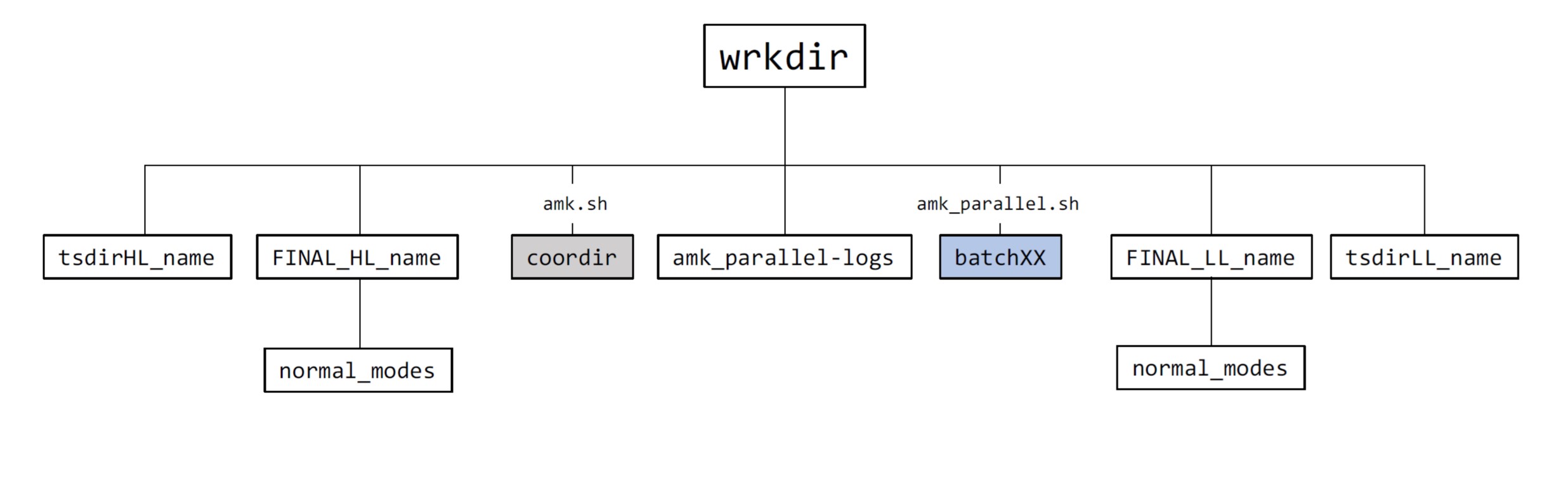
The figure below shows the main folders that are generated in wrkdir. Folders batchXX, where XX = 1 - tasks, are generated with amk_parallel.sh. This script is also invoked by llcalcs.sh, and when that happens these folders are temporary,i.e., they are removed at the end of the tasks. Directory coordir is only generated in those directories where amk.sh is executed. The amk_parallel-logs directory contains a series of files that give information on CPU time consumption for the different calculation steps when they were executed with GNU Parallel. Directories tsdirLL_name and tsdir_HL_name are generated at runtime and are employed to generate the final files and directories. For that reason, they should not be removed. Finally, the most important files are gathered in a final directory (FINALDIR) which is named after the system’s name: FINAL_level_name, with level being LL for low-level or HL for high level; see figure below.
Relevant information
Scripts final.sh and FINAL.sh are employed to collect all relevant information in FINALDIR. These folders contain files as well as a subdirectory called normal_modes, which includes, for each structure, a file in MOLDEN format with which you can visualize the corresponding normal modes. The files included in these folders are the following.
convergence.txt
This file lists the number of located transition states as a function of the number of trajectories and iteration (Only in FINAL_LL_FA).
frag_warnings
This ifle contains information on failed ab initio calculations of the fragments. If all calculations are successful, the file is absent. The file is located in FINAL_HL_FA folder.
MINinfo
This file contains information of the minima:
MIN # DE(kcal/mol)
    1    -8.341
    2     0.000
    3     5.288
    4     6.732
    5    15.441
    6    82.122
    7   110.400
    8   188.254
Conformational isomers are listed in the same line:
1 2
3 4 5
TSinfo
Likewise, this file contains information of the TSs:
TS # DE(kcal/mol)
   1    -1.624
   2     1.868
   3     9.644
   4    25.135
   5    32.821
   6    37.608
   7    40.956
   8    44.037
   9    53.173
  10    58.156
  11    60.015
  12    85.659
  13   142.228
  14   188.765
  15   191.650
Conformational isomers are listed in the same line:
9 11
In the above files, DE is the energy relative to that of the main structure specified in the FA.dat file optimized with the semiempirical Hamiltonian. The integers are used to identify, independently, minima and transition states. Notice that, in this example, MIN 2 corresponds to the structure specified in FA.xyz.
table.db
These are SQLite3 tables containing the geometries, energies and frequencies of minima, products and TSs, respectively: table can be min, prod and ts, which refer to the minima, product fragments and transition states, respectively.The different properties can be obtained using select.sh:
select.sh FINALDIR property table label
where property can be: natom, name, energy, zpe, g, geom, freq, formula (only for prod) or all, and label is one of the numbers shown in RXNet below, which are employed to label each structure. At the semiempirical level, the energy values correspond to heats of formation. For high-level calculations, the tables collect the electronic energies. Please note that for the hybrid calculations involved through the use of keyword LowLevel_TSopt, energies, zpe and frequencies in the tables are those obtained with MOPAC, while the geometry in ts.db is the one obtained at the g09/g16 level of theory.
As an example, to obtain the geometry of the first low-level transition state of FA, you should use:
select.sh FINAL_LL_FA geom ts 1
MOPAC optimizations of minimum-energy structures might not be fully optimized and, consequently, imaginary frequencies might arise for minima. Additionally, the frequencies obtained for fragments prod are meaningless as these structures are not optimized.
RXNet
This file contains information of the complete reaction network, that is all the elementary reactions found by the amk program; the file shown below, and the following ones, were cut and show only up to TS 15.
TS # DE(kcal/mol)    Reaction path information
==== ============    =========================
   1      -1.6 PR2: CO + H2O <---> PR2: CO + H2O
   2       1.9         MIN 1 <---> MIN 2
   3       9.6         MIN 3 <---> MIN 4
   4      25.1         MIN 1 <---> MIN 1
   5      32.8 PR2: CO + H2O <---> PR1: H2 + CO2
   6      37.6         MIN 4 ----> PR2: CO + H2O
   7      41.0         MIN 1 ----> PR2: CO + H2O
   8      44.0 PR1: H2 + CO2 <---> PR1: H2 + CO2
   9      53.2         MIN 1 <---> MIN 4
  10      58.2         MIN 2 ----> PR1: H2 + CO2
  11      60.0         MIN 2 <---> MIN 5
  12      85.7         MIN 2 <---> MIN 6
  13     142.2         MIN 3 <---> MIN 6
  14     188.8         MIN 2 <---> MIN 8
  15     191.7         MIN 7 <---> MIN 8
As can be seen, for each transition state, this file specifies the associated minima and/or product fragments and their corresponding identification numbers. Notice that TS, MIN and PR have independent identification numbers.
As indicated in the General section , you can use the keyword HL_rxn_network to significantly reduce the number of TSs to be reoptimized in the HL calculations and therefore the reaction network.
By using the keyword like this:
HL_rxn_network reduced
TSs associated to PR <---> PR steps (i.e., bimolecular reactions) and interconversions between optical isomers will not be reoptimized in the HL calculations.
You may include a number as a third argument:
HL_rxn_network reduced 55
In this case, not only TSs associated to bimolecular reactions and interconversions between optical isomers, but also TSs having relative energies larger than 55 kcal/mol will not be considered for HL optimizations, i.e., they will not be included in the HL reaction network. We notice that the last argument must be an integer.
Another useful keyword for reducing the number of high-level calculations is Energy in the Kinetics section
RXNet.barrless
Barrierless reactions are included in this file; only when MOPAC and g09/g16 are employed. The user must be aware that the channels are those consistent with the values of the keyword neighbors explained above. These channels are not considered in the kinetics, but they are plotted in the complete graph indicated below.
TS #   DE(kcal/mol)      Reaction path information
====   ============      =========================
1          152.8         MIN 1 ----> PR6: HO + CHO
2          170.4         MIN 3 ----> PR7: HO + CHO
3          150.6         MIN 6 ----> PR8: HO + CHO
Here TS refers to a dynamical TS and no saddle point exists in these paths.
RXNet.cg
By default, see below, the KMC calculations are “coarse-grained”, that is, conformational isomers form a single state, which is taken as the lowest energy isomer. Such reaction network, which also removes bimolecular channels, is the following:
TS # DE(kcal/mol)    Reaction path information
==== ============    =========================
   6      37.6      MIN 3 ----> PR2: CO + H2O     CONN
   7      41.0      MIN 1 ----> PR2: CO + H2O     CONN
   9      53.2      MIN 1 <---> MIN 3             CONN
  10      58.2      MIN 1 ----> PR1: H2 + CO2     CONN
  11      60.0      MIN 1 <---> MIN 3             CONN
  12      85.7      MIN 1 <---> MIN 6             CONN
  13     142.2      MIN 3 <---> MIN 6             CONN
  14     188.8      MIN 1 <---> MIN 8          DISCONN
  15     191.7      MIN 7 <---> MIN 8          DISCONN
The last column with the flag “CONN” or “DISCONN” indicates whether the given process is connected with the others, CONN, or whether it is isolated, DISCONN. This flag is useful when you choose a starting intermediate for the KMC simulations, because that intermediate should be connected. If you want to include all conformational isomers explicitly in the KMC simulations, you need to construct the reaction network by using the allstates option, as described in the next section.
RXNet.rel
This ifle is similar to RXNet.cg, but only collects the relevant paths, that is, those included in the Energy_profile.pdf file. A maximum of 100 TSs are printed in this file. If this number is reached, both Energy_profile.pdf and RXNet.rel would be incomplete, and the pathways drawn in Energy_profile.pdf could be less than those that appear in RXNet.rel.
rxn_x.txt $\scriptstyle{(}$x = all, kin$\scriptstyle{)}$
Each line of rxn_all.txt lists the nodes, first two columns, and the weight, last column, which is the number of paths connecting the two nodes. For rxn_kin.txt the weight is the total flux in the kinetics simulations.
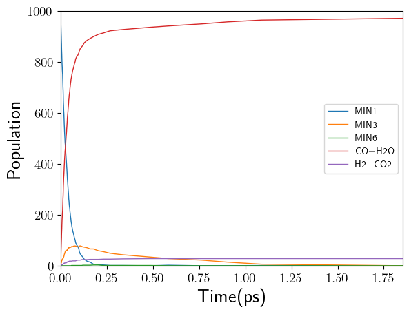
kinetics.csv
This file includes the population data for each species over time. To simplify the process of generating a plot from this file, we have used a CSV format that can be used with pandas and matplotlib to create a figure like this:
This Notebook shows how to build the plot using pandas and matplotlib. This is the code snippet:
!sudo apt install cm-super dvipng texlive-latex-extra texlive-latex-recommended

import pandas as pd
from matplotlib import pyplot

pyplot.rcParams['text.usetex'] = True
pyplot.xticks(fontsize=14)
pyplot.yticks(fontsize=14)

data = pd.read_csv('kinetics.csv')
for count,col in enumerate(data.columns):
  if count == 0:
    x=data[col]
    xcol=col
  if count >=1: pyplot.plot(x,data[col],label=col,linewidth=1.0)

pyplot.ylabel('Population',fontsize=20)
pyplot.xlabel(xcol,fontsize=20)

pyplot.legend()
pyplot.xlim(0,max(x))
pyplot.ylim(0,1000)
pyplot.tight_layout()
pyplot.savefig('kinetics.png')
pyplot.show()